A visit to a Random Forest:

image source

In machine learning, an ensemble method is one that uses a couple of different algorithms together to achieve better results than that of a single method. A random forest is one of those. As the name suggests, it's made up of a bunch of trees - decision trees, that is. I used this algorithm on a project and thought I'd share on a high level what they are and how they can work, and how to tell if you have a decent model.

Let's start with a single tree. A decision tree is considered to be what's called 'supervised learning' since we have a sample of data where we know what the value for the target is. A decision tree takes in data, including the target, and makes 'decisions' to break it down into more and more simplified variables or 'leaves' that align with the target values. It uses these variables to make predictions using various random data selection as input - see how the randomness fits in? The more 'votes' cast by these predictions that inform the strength of the learning. Confused? Let's try a different explanation.

A very simplified example may be asking your friends what their favorite restaurant is. My model was binomial, so we'd ask them if you should go to restaurant 'a' or restaurant 'b'. In this case, the target is a favorite restaurant. Each friend represents a tree and like different friends are, take in different (random) data and some may ask more than one question - like "What kind of food do you like?" and "Do you feel like sitting down or taking out?" or "How hungry are you?". Each friend makes a suggestion based on your responses. These votes aggregated would represent a forest, and the varying questions or features used to evaluate the target are the random part. The more votes a certain restaurant gets the higher the suggestion. If everyone votes for the same restaurant you've achieved the lowest level of uncertainty or entropy. What we look for in a random forest are those splits that are biased towards low entropy.

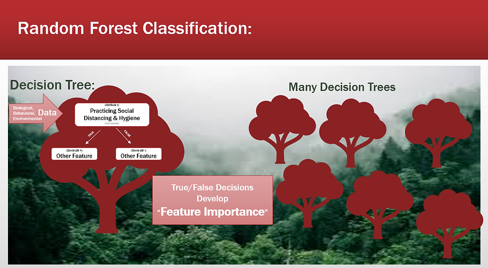
In the example below, I try to show how biological, behavioral, and environmental data collected from a self-reporting tool by a company called Nexoid in the United Kingdom. This data was collected in April of 2020 when the covid-19 pandemic was relatively 'new'. The tree below uses a feature for the self-assessed risk in terms of behavior like practicing social distancing and hygiene were being practiced. Based on the outcome, it evaluated another feature, and so forth and so on.

Ultimately the trees 'vote' and using feedback develop feature importance.

Feature importance is the score assigned to each of the features in relation to how meaningful or helpful they are in making predictions. Feature Importance can give us insight into the data, and the model. Since we seek the lowest entropy, you can imagine the more simple the dataset the lower the entropy and more confidence we can have in our prediction.

In the dataset I collected for this project, there were 43 features on the varying factors I mention above. This includes the target which is in this project was 'covid19_positve'. For this target, a value of 0 indicates that the person did not test positive, and 1 indicates they did. Since we are looking to 'weed out' irrelevant or other features that might interfere with getting a clear classification, we try to eliminate unuseful features or those that might otherwise increase entropy. In the case of what restaurant a or b, an unuseful feature might be if you are wearing socks or not.

The idea for this project was to accurately use a classification algorithm to predict if someone would test positive. I could use the results to indicate which of these factors were important to have a result of someone testing positive. After I imported the dataset and began to evaluate which features that could or should be dropped. One way to do this is to find out if they were highly correlated or related to the target they are, so I created a data frame that found these correlations:

df_cor = pd.DataFrame(df.corr()['covid19_positive'].sort_values(ascending=False))
df_cor

Naturally, the target was perfectly correlated but none of the other features in the initial scan seemed to show enough correlation to warrant dropping them for that purpose alone.

I did end up dropping some features that were sparsely populated and others for a variety of reasons.

I used scikit learn's RandomForest Classifier for many reasons - but mainly because of the usability and reporting capabilities that can readily illustrate feature importance. Various attempts were used to attempt to predict whether an individual would test positive for COVID-19 and baseline classification testing was run using the following models:

* Decision Trees

* Random Forest

* XGBoost

Something I've failed to mention up until now is that this data had an extremely imbalanced target to classify. Out of the 575,210 samples I ended up using, only 791 tested positive! That's .13%! This means that to train the model to identify the people who didn't test positive, we have tons of data. For those that did... it's a tiny amount to try to learn, and it's ultimately the problem we're trying to solve. Unbalanced data is something I seem to run into frequently. The world is an imperfect place, after all. I talk about each here in another blog... this is its own world. The main reason I'm sharing this is that I talk about how to evaluate models next, and mine wasn't stellar, but this imbalanced data ended up as ultimately the main problem to solve for this project.

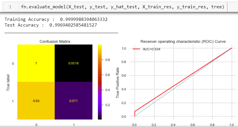
I wrote a function called evaluate_model to help evaluate the binary classification models. This gave me the training and testing accuracy and provided visuals to help me find how often the model forecasted the actuals. One of these visuals is called a confusion matrix. These illustrate what we've become too familiar with since covid19 reared its head - true positive and true negatives. True positives are those that the model predicted to be in the target class. True negatives are those that the model predicted to not be in the target class. True negative rates are shown in the upper left-hand corner and true positives in the lower right. Also, I visualized the Area Under the Curve or AUC to compare these true positive rates versus true negative rates. I won't take you super deep into this, but for a simplistic explanation, if the plot aligns with the diagonal line, it would demonstrate that my model is a random classifier (a coin flip) - anything below the horizontal line represents worse than just chance. The more this line is drawn towards the upper corner, the better job the classifier is doing.

My initial model(s) left much to be desired and are a great place to start in evaluating things.

We can see that while this first is a SUPER accurate model, it's because of the super high True Negative rate... all that data that shows very accurately who doesn't test positive. What we're interested in here is the True Positive Rate... which is... 7% of the time... blech! ...and the AUC... ya... it's pretty much just random classification happening:

I'll spare you the entire process but out of the three classification models, my baseline random forest showed the most promise...so I began to 'tune' it. You can see here that the Test Accuracy is higher than my Training Accuracy. This is a result of 'overtraining' or 'overfitting' your model.

I like how Andrew Gelmen puts it here: "Overfitting is when you have a complicated model that gives worse predictions, on average, than a simpler model."

This model still needed work:

There are many hyperparameters for tuning sckitlearns RandomForestClassifier. The ones I spent most of my time on were:

*n_estimators - how many trees you want in your forest

* criterion= this assigns your algorithm to use, either 'gini' or 'entropy' - both evaluate how pure each node is and I like how it's explained here. I tried both in various iterations

* max_depth=how deep you want each tree to go

* max_features=The number of features to consider when looking for the best split

* class_weight=This feature allows you to weight a class. The “balanced” mode uses the values of y to automatically adjust weights inversely proportional to class frequencies in the input data. This ultimately came in handy after I tried various methods for addressing the hyperimbalance.

There are ways you can adjust each of these, and I can go deep in how to tune these in another post. For the most part, I used trial and error and/or by using a package that will do the work for you using GridSearchcv. I ultimately gave up on this since some models were taking over 20 hours to run and I was running out of time.

Through trial and error I was able to manually tune my forest;

time = fn.Timer()
time.start()
rf_clf8 = RandomForestClassifier(criterion='gini', max_depth=2, max_features=.45, class_weight='balanced',n_estimators=80, random_state=111)
rf_clf8.fit(X_train, y_train)
time.stop()

[i] Timer started at05/11/20 - 09:33 AM
[i] Timer ended at 05/11/20 - 09:34 AM
- Total time = 0:01:19.461404

it still took an hour to run this one classifier, but I was able to get the true positive rate up by 57% and AUC/ROC score to improve by .34~!

Remember how I talked about feature importance? Using sckit.learn's RandomForest .feature_importance() function and another function I built to visualize it, this model identifies the following:

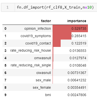
Again, I won't go into deep detail here, but the higher the score for feature importance, the more important the feature is. It makes sense that the top feature was one that captured whether the participant thought they were infected ranked high, that they had symptoms and had come into contact were the top three. This isn't surprising, but it illustrates the point of how the model works.

The model still could use work, but I was proud of making progress considering the hyperimbalance. I wonder what would happen if I used an updated version, and dove deeper into hyperparameter tuning. Challenge me or drop a comment for ideas and inspo.

If you're interested, the link to this project can be found here

More reading on feature importance can be found here