Tableau: It's not just for visuals - Trend Lines, R-squared, and P-values oh my! Was that a model?

I've been practicing data science and analytics using libraries like scikit-learn's KMeans, Statsmodels Linear Regression, and matplotlib for analytics and visualization (among many others). I spent time studying the maths behind the tools and packages as well as learning to code in Python in order to use Pandas and Numpy to preprocess the data - to clean, merge, and get data into one place to leverage the powerful tools. Data can come from more than one data source so this part can be tricky. Sometimes when collecting data it comes from several sources and formats and it's necessary to spend a lot of time on this part. All of this is a lot.

More recently, I've found myself using Tableau more often since the usability and powerful analytics tend to speed up many of these processes in a way that's visual and easily consumable. As I mention in this post, bringing datasets together from various formats is facilitated in a way that is really unique. In Tableau, it's possible to join a SQL query with a static excel spreadsheet. Data can be aggregated, calculated and visualized by dragging and dropping rather than importing and converting, and coding. Even more recently, I've been exploring the analytics capabilities like KMeans Clustering.

Building on the merging as well as the analytics, with the understanding of the mathematic and statistical values, I was able to go deeper into the analysis.

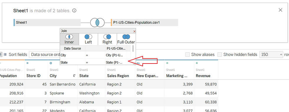
I picked up on a project where I was looking at revenue and marketing spend and had just discovered the KMeans clustering capabilities. After bringing in the initial data provided, an additional text file was imported as a .csv file with census information on the cities to provide additional insight. The two tables were joined on the physical layer.

In my personal analysis process, I use a methodology where I Obtain, Scrub, Explore, Model, and obtain and share iNsight - or OSEMN. On this project, I'd obtained the data (an excel spreadsheet), but now I joined it with a different file type (.csv or text file). Staying on task, it was time to scrub it or make sure it was 'clean' - had no duplicates, null values and it 'made sense'. My original dataset had 150 rows, and after the join had 159. When the number of rows increases after a join, it can indicate duplicates have been generated. One way to resolve this is to examine the table and manually remove duplicates. 150 rows is relatively small - but still is tedious. Another way could be to add another layer of granularity in the join. Duplicates happen a lot with geographic data since cities can be named the same thing in different states or countries. Luckily both tables had city and state, so I could map them to each other to help identify unique cities. By adding the second level of granularity I was able to get the 150 rows - see how I added 'State'?

With this new join, I was able to re-create my clusters by comparing revenue with market spend and breaking it down by location (store number) to get the scatter plot:

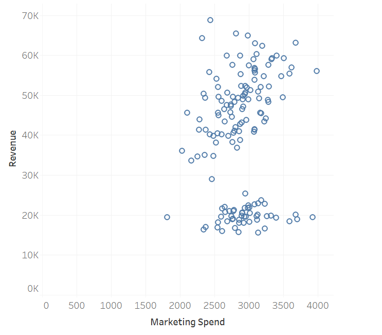
you can see how the clusters are forming, and by clicking on the analytics tab as I'd done before, I clicked and dragged the clusters into the plot and the mathematic calculations around similarity took place behind the scenes and divided these clusters visually.

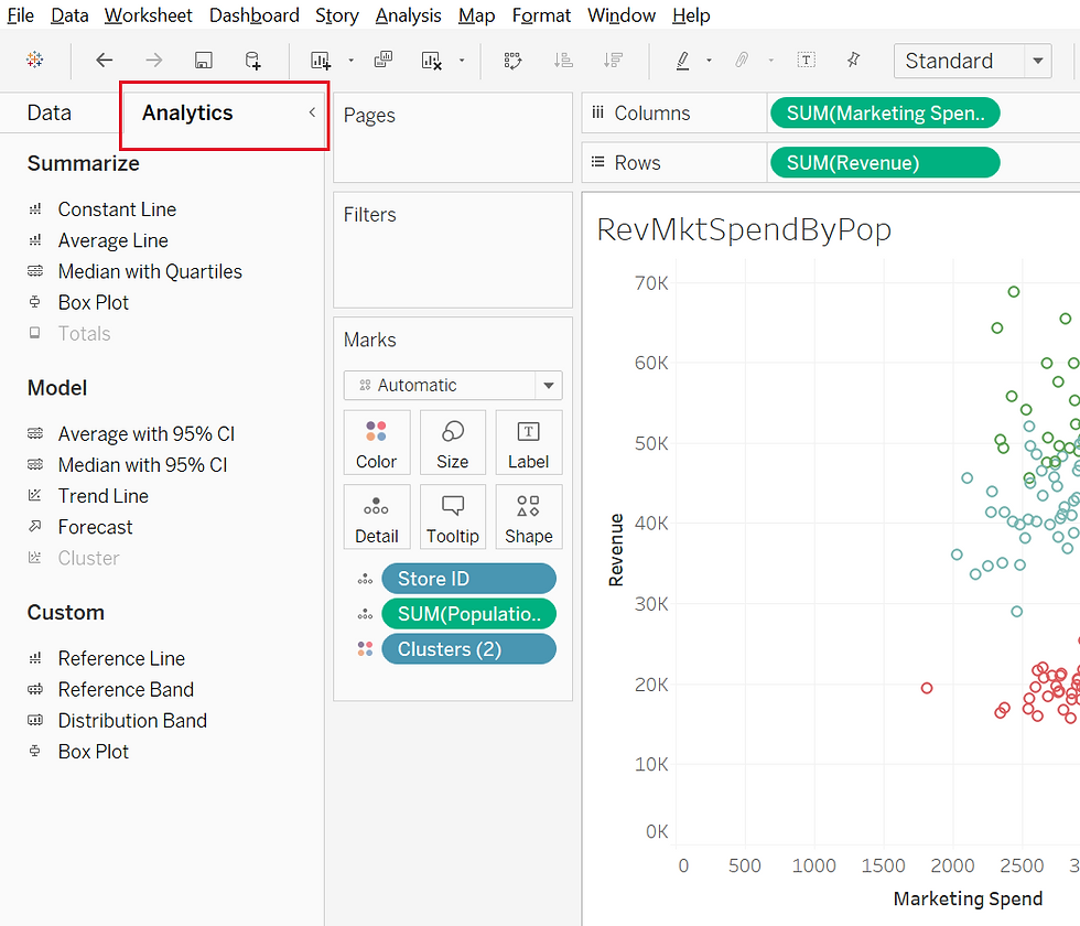
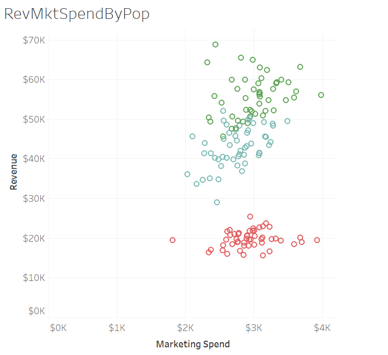
I was able to edit the clusters and drag in population to add a different dimension. Once I dragged the population into detail, another level of analysis could occur. Visually, it was great. Three clusters appeared and the population detail demonstrates three levels of return on marketing investment as well as relative population information. On my worksheet, if you hover over a data point, the population is revealed. Trends are starting to show up. Those in the red cluster revealed a population around 100K or less, those in the blue 100K or more, and those in the green, even higher. You might begin to think yes! We've cracked the code. The larger the population, the higher the return on marketing investment.

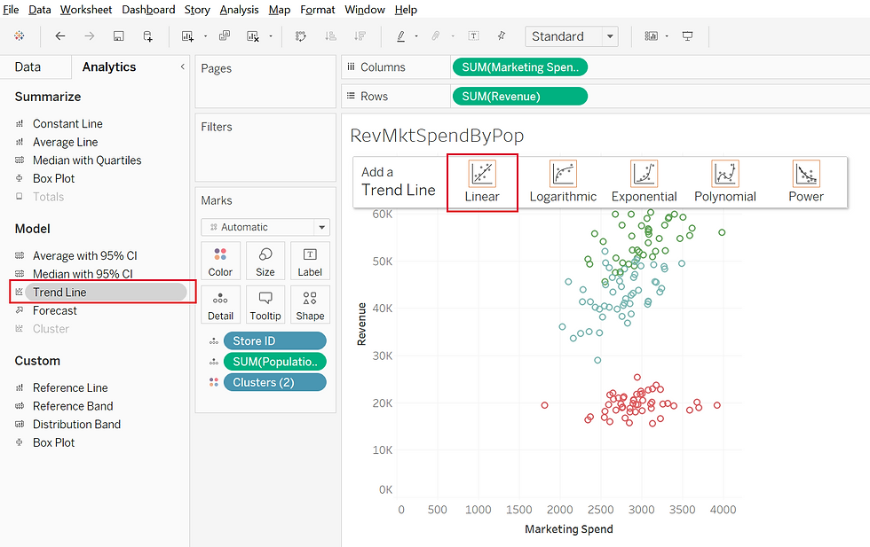
I thought so too.... until I started using the trendlines. The modeling piece is taken up a notch for me - I love learning what Tableau can do!

On the Analytics tab, I clicked on trend lines and saw a good old-fashioned linear regression line... AND Log, Exponential, Polynomial, and Power... each I'd used in past projects for their various capabilities. Since we were looking at financial modeling an exponent of a linear regression would represent return on investment.

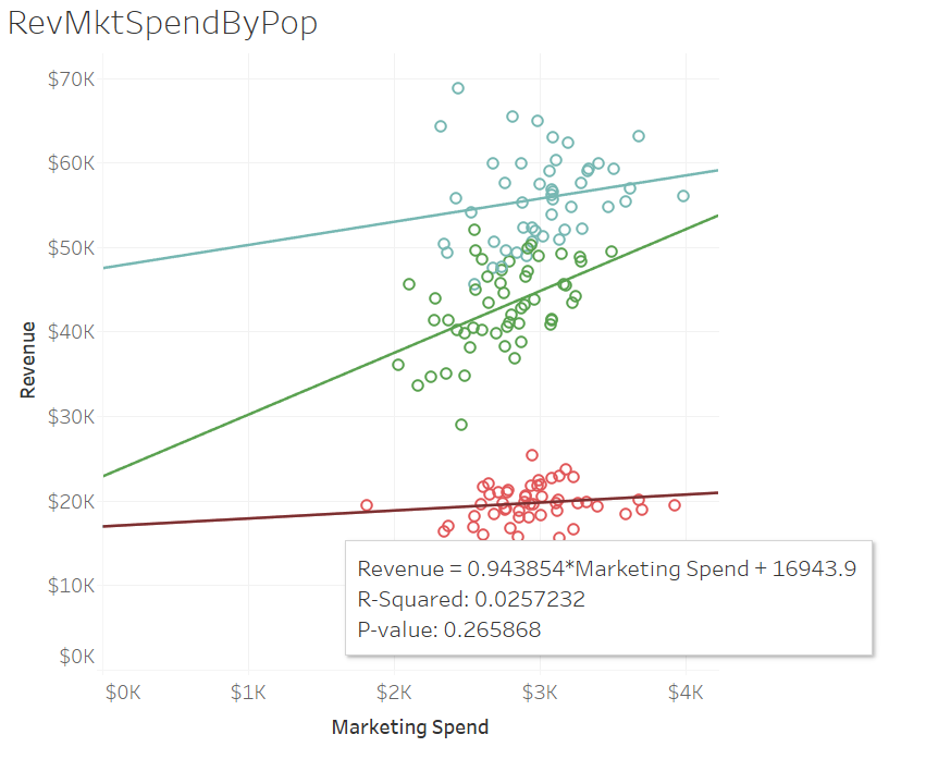
Look at that - The value below reflects the coefficient of that trend line for the bottom cluster and shows us that for every dollar we spend in marketing, we get $.94 in revenue (we lose $.06)

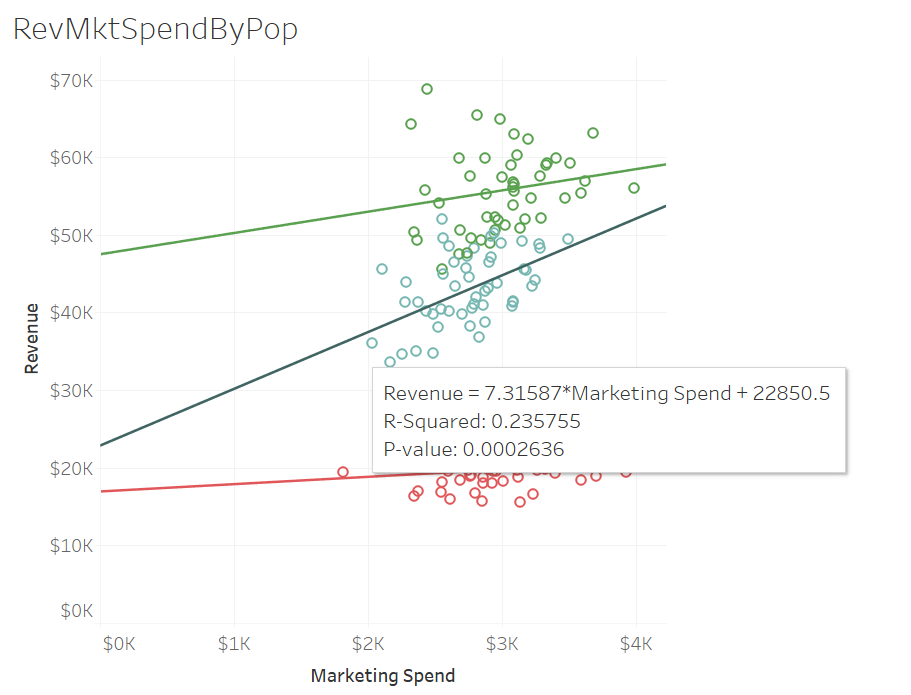
For the mid-range population - it proved to be a much better yield: For every dollar spent a return of $7.32 was modeled.

...and the higher population was $2.74.

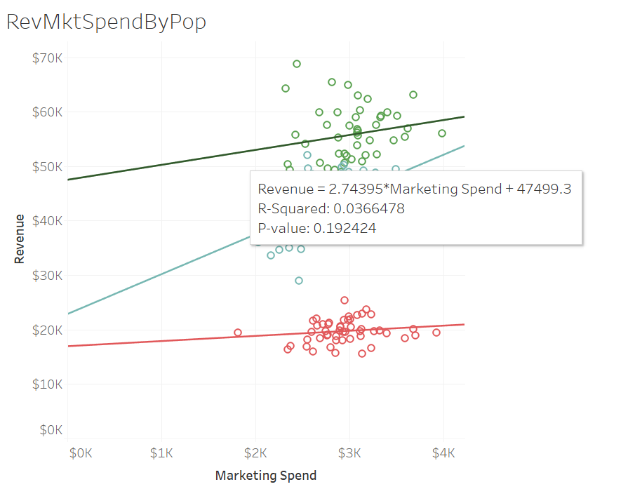
The other metrics that are shown are:

R-Squared which measures the difference between where the values lie versus the trend line all added up and squared. It shows how much variance in revenue could be accounted for based on the marketing spend - or how well the line fits.

and

P-Value - or the probability that this is due to chance - the smaller the number the more likely it is NOT due to chance. You'll hear this a lot in analysis that it has significance.

If you click on the trend line and ask it to describe the model...you can get a lot more detail... A LOT:

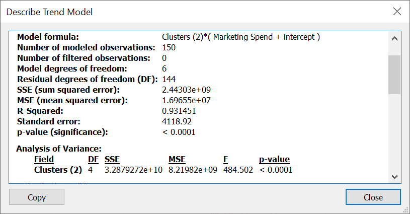
In a previous analysis, it was determined that there were factors that affected return on marketing spend. By adding a highlighting feature, we were able to visualize that newer stores belonged to the higher yield cluster, as well as those in certain states.

By understanding what kind of business this was (it's a direct service offering) and adding the observation of population in conjunction with the trend lines we were able to develop a linear regression model that helped to identify the highest yielding return on investment. By adding these features, it was discovered that in general, populations of 100K or less predict a loss on marketing spend. That those in the largest populations do better, but those in the middle range tend to do the best.

I love a good visualization as well as useability, but discovering that Tableau can also add analytics to me makes me like it even more as a tool.

Did you know it could do that??