Time Series.... is really a Series.

When looking at data in relation to time, we hear this phrase: Time Series. Time series looks at how time affects a value. It's used for analysis, but the main purpose is to predict future values. Many predictive models exist without being time-dependant. But pretty much any predictive model that takes into account time at regular intervals can use time as an independent variable and makes it a candidate for time series.

Examples of time series problems:

• Seasonal Sales

• Daily, Monthly, or Yearly Temperatures

• Traffic

• Finance

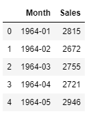
To answer a question, data is captured at regular intervals and ordered chronologically. I'm using champagne sales from 1964 to 1973 as an example:

#importing pandas and dataset
import pandas as pd

#creating a dataframe from the csv file 
df = pd.read_csv("https://raw.githubusercontent.com/jbrownlee/Datasets/master/monthly_champagne_sales.csv")

#making sure it loaded and take a first look 
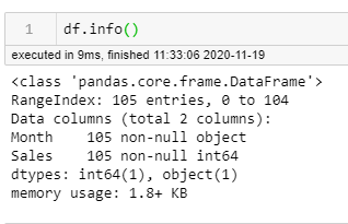
df.head()

Here's the top of the data frame and the information describing it. Additionally, we can see we're dealing with 105 months. Sales are reported in integers - easy enough for Pandas and other functions to use, but see how Month is read here as an object?

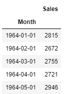
Since this is a time series, two things need to be done:

1) We need to convert Month into datetime

2) We need to set the time ('Month') as the index

#changing Month to datetime
datetime = pd.to_datetime(df['Month'])

#setting the index to be datetime
df.index = datetime

#getting rid of the 'old'column-Month that is now the index
df.drop(columns="Month", inplace=True)

.... and then turn it into an actual Series or an index and one column or series. In Pandas, it's pretty easy:

#creating a timeseries using sales and dates
ts = pd.Series(df['Sales'].values, index=datetime)

Then let's take a first look at our values against a timeline:

import matplotlib.pyplot as plt
#a quick look for patterns:
ts.plot()
plt.show()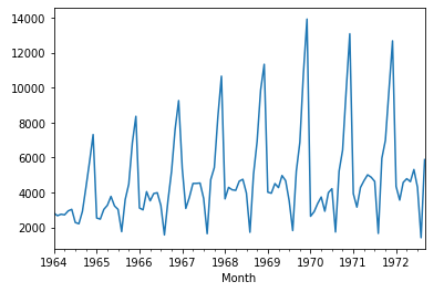

Yep. There are some definite patterns here. The main components of time series forecasting are:

• Noise - this one is just random variability. No clear pattern, no reason just 'noise' or random up and down movement. Not a lot of noise above. This plot demonstrates more of the next two:

• Seasonality- Predictable patterns that occur at regular intervals. It is pretty cliche that champagne sales increase in December for the holidays and this proves it for 1964 to 1972.

• Trend- long term movements. In our champagne sales, you can see an upward trend from 1964 to 1970. See how the peaks continue a pattern that goes upwards?

• Cyclical Components - These are longer-term patterns that seasonality (years, decades) and aren't necessarily predictable but illustrate external conditions.

So we can see just with an initial plot seasonality and some trends. But what if it's not super easy to eyeball? What if the data is all on top of each other and you need to know for sure? The answer: A Dickey-Fuller Test. (we use an augmented one) Basically, this test assumes (aka null hypothesis) that a unit root is present - or a systematic pattern that is unpredictable. Alternatively, the data are non-stationary - or have means, variances, and covariances that change over time so they cannot be modeled or forecasted.

If we reject the null hypothesis, the time series is not stationary - we can often transform it to stationarity with one of the following techniques:

• Differencing - by subtracting the previous observation from the current observation. This has the effect of removing or minimizing a trend without moving seasonality. This really helps to find true correlations. I'm sorry to go on and on about this one, but it does the trick more often than not, and this particular method we'll talk about more later.

• Log - assigning the log value to normalize the original values - equally distributing the values.

• Subtracting the rolling mean from each value to smooth out the wave

• Subtracting the exponentially weighted rolling mean from each value doing the same thing as above, but adding weight to more recent data. This smooths out the waves, too but in my opinion, honors more about what's going on more recently.

Another way to evaluate what's going on and even find a way to combat non-stationarity is through seasonal decomposition. Below, you can see the various aspects of the data. It's also helpful to use this to apply it to whatever problem you're trying to solve. Are we looking to see if champagne sales increase overall over time, or are we trying to manage production to meet the needs of seasonal demand?

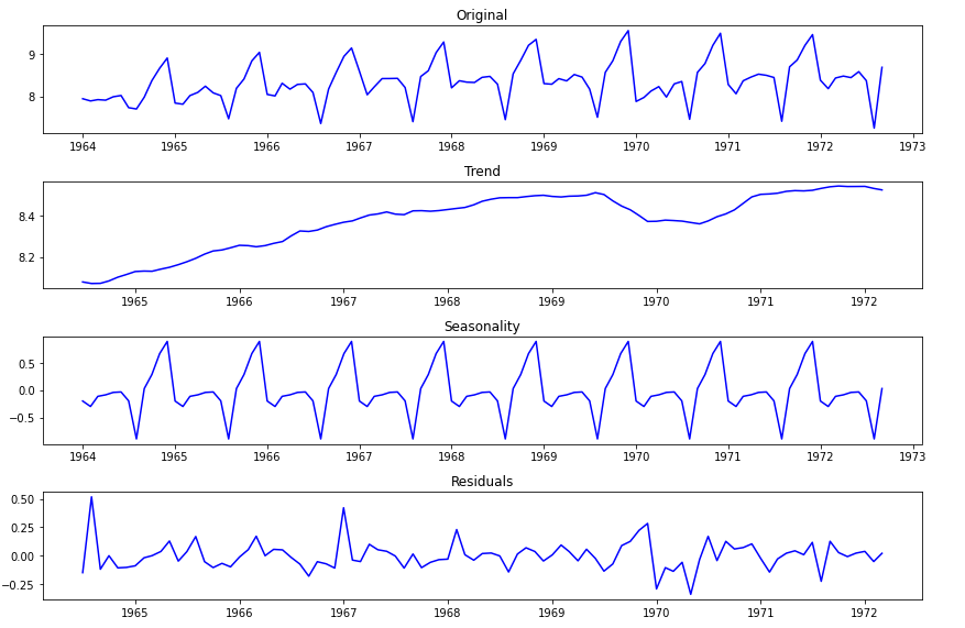
All of these methods help to remove trends and find a true correlation between values, hence being able to predict future values.

Autocorrelation is a very powerful tool for time series analysis. It helps us study how each time series observation is related to its recent (or not so recent) past. Processes with greater autocorrelation are more predictable than those without any form of autocorrelation.

Shifting gears slightly..

One simple way we can ou can use the .shift() method in pandas to shift the index forward, or backward. When we shift the data forwards or backward, it's easy to identify where the series is correlated to itself. Here, what we can see with our naked eye is revealed to be true:

#setting the number of shifts to 36 mos
total_shifts = 36

#creating each occurance of one shift up to 36 mos:
shifts = (ts.shift(x).rename(f'Sales shifted{x}') for x in range(total_shifts))

#creating a series of each shift for 36 months
res = pd.concat(shifts, axis=1)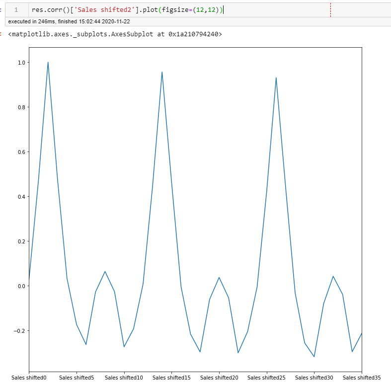

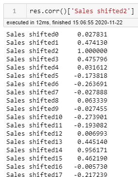
You can see here the high correlations happening every 12 months when we plot it. This is confirmed when we look at the values every 12 months as well. When we create a shift of 2, the value at 14 is the highest, 12 months away. Also notable is the sub correlation every 6 months which wasn't as noticeable on the first plot (see 8 shift value):

Back to autocorrelation which does this using these shifts or lags to reveal seasonality of data. Pandas has a nice package you can use too, to show this. See how the plot looks much like the one above?

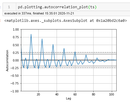
When we look at the plot above, we can see that there are 6 lags (the first one is right at 0 and might be unnoticeable) that occur before the lines fall within the confidence interval lines (dashed and solid lines) ... this indicates that a lag of 6 is significant.

All of this leads us up to ARIMA Models:

An autoregressive (AR) model is when a value from a time series is regressed on previous values from the same time series. It uses a constant and yesterday's noise (random up and down movement) to predict future values:

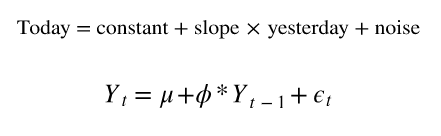
It's essentially a linear regression that uses a constant + a co-efficient (phi) which is multiplied by a timestep (t-1) and added to the noise. The order is how many of these coefficients we use - or how many series we use. If the constant or average is 0 - it's called a white noise model. If the mean is not zero, it means the time series is autocorrelated.

A moving average (MA) model uses the weighted sum of today's and yesterday's noise to help predict future values.

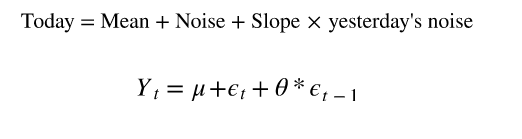
We still have a co-efficient (theta) that corresponds to one timestamp before. In this case, it's multiplied with it, and the noise is added prior to making this calculation. The same is true for the order and mean. In this case, however, if the slope is not 0, the time series is autocorrelated and depends on the previous white noise process.

So we have the AR + the MA. When we add in differencing to these two, we have ARIMA which I will cover in my next post. For now, we have the basis for what we need to predict future values that are dependant on time. On a high level, this is all you have to do:

• Detrend the time series (my fave is by using differencing). ARMA models represent stationary processes, so we have to make sure there are no trends in our time series

• Look at autocorrelation and in some cases partial autocorrelation of the time series

• Decide on the AR, MA, and order of these models

• Fit the model to get the correct parameters and use for prediction.

In my next blog, I'll do just that. All in good time.