Collecting meaning from words with Linear Support Vector Classification

I am new to natural language processing (NLP). In a project I'm revisiting, I classified negative and positive reviews and then used cluster analysis to identify patterns to inform next-generation product development.

A little background:

I got the data from a site called App Annie. It is a decision-making platform for the mobile app economy. App Annie combines the analytics of one's own apps with a granular understanding of the competition and market to provide a unique 360-degree view of one's mobile business. In short, it takes consumer data and 'ranks' apps. It was used in combination with google play scraper to obtain the data for this project. I was looking to find:

Questions to be answered:

• What are the top-grossing health and wellness apps?

• What's in a positive review versus a negative review?

• What insight can be gleaned from reviews to provide business intelligence for next-gen apps?

I'm not going to address the scraping or the top-grossing health and wellness apps here - I can do that another time or if you want to see the project go here:

I remembered the outcome - the part where I used Latent Dirichlet Allocation to examine what patterns existed in positive and negative reviews. It was insightful. I wrote a blog about that here. But, in the post, I glean over how I classified the positive and negative reviews in the first place.

From the fifty thousand reviews, I grouped the good(5 stars) and bad(1 star) reviews. The other reviews I labeled as 'neutral'.

stars_dict = {5:'good', 4:'neutral', 3: 'neutral', 2:'neutral', 1:'bad'}
clean_df['Target'] = clean_df['score'].map(stars_dict)

The 'content' field contained the text data of reviews that had been pre-processed. I took out stopwords or words like 'a', 'the', 'and', removed punctuation, and lemmatized them.

I did this through a couple of preprocessing steps:

#pulling the strings together
clean_df['content'] = clean_df['content'].apply(lambda x: ' '.join(x))

which involved a function that did all the stuff in the paragraph above called .clean_tokens()

def clean_tokens(text):
    '''A pre-processing function that cleans text of stopwords, punctuation and capitalization, tokenizes, lemmatizes
    then finds the most frequently used 100 words
    
    text - the text to be cleaned in string format'''

    # Get all the stop words in the English language
    import nltk
    from nltk.corpus import stopwords
    #importing additional function to execute
    import string
    #importing and enstantiating lemmatizer 
    from nltk.stem import WordNetLemmatizer
    lemmatizer = nltk.stem.WordNetLemmatizer()
    
    stopwords_list = stopwords.words('english')

    #remove punctuation
    stopwords_list += list(string.punctuation)
    ##adding adhoc all strings that don't appear to contribute, added 'article, page and wikipedia' iteratively as 
    ##these are parts of most comment strings
    stopwords_list += ("''","``", "n't", 'app', "...", "n't",
                       "wa","ve", "ha","'", 'wa', 'ha', 'ca', "'ll",
                       'doe' 'wo','u',"'s","'ve", "ve","'m","wo","doe",
                       "'ve", "'d") 
  
    
    from nltk import word_tokenize
    tokens = word_tokenize(text)
    lemma_tokens = [lemmatizer.lemmatize(token) for token in tokens]
    stopped_tokens = [w.lower() for w in lemma_tokens if w.lower() not in stopwords_list]
    return stopped_tokens

clean_df['content'] = clean_df['content'].apply(fn.clean_tokens)

Then I split the target from the data and assigned it to the variable y. The target is what we are trying to predict or classify so our target was good, bad, or neutral in this case. The clean_tokens function cleans up each word but they come out as separate values so I had to put them back together again using .join()

X = clean_df['content'].apply(lambda x: ' '.join(x))
y = clean_df['Target']

For classification, you need to split your data into two parts, training and testing. This way you can compare what your model predicts(train) to actual results(test). In the case below, I'm using 70% of the data to train my model and 30% to test it:

X_train, X_test, y_train, y_test = train_test_split(X,y, test_size=.3, random_state=2)

Linear Support Vector Classification:

There is no one silver bullet when it comes to classifying something. One algorithm might be great at classifying a target (how something is labeled ) and be horrible when applying it in another case. You should try different algorithms when you can to see if one works better. In this case, I tried a multinomial Bayes, Logistic Regression, and linear Support Vector Classification. It's theorized that the best model for NLP is Linear Support Vector Machine, and compared to the other two, it was true.

For NLP you vectorize the text data - you turn it into numeric data - then feed it into the classification algorithm. I use a pipeline to do this in one step:

from sklearn.pipeline import Pipeline
from sklearn.svm import LinearSVC

weights = {'good':.4, 'bad':.4, 'neutral':.25}

lSVC = Pipeline([('tfidf', TfidfVectorizer()),
                ('clf', LinearSVC(dual=False, multi_class='ovr',C=.7,
                                  random_state=42,class_weight= weights,
                                  max_iter=6)),
               ])
lSVC.fit(X_train, y_train)

Once the model is fit and evaluated, we can extract the scaling and classification components from the pipeline using .named_steps()

lSVCscaler = lSVC.named_steps['tfidf']
lSVCclassifier = lSVC.named_steps['clf']

I like building functions that I might use in the future or for code that is repetitive. This was one of my favorites from this project. It gave me insight into what words had the most important in terms of classifying text as 'good' or 'bad'.

The function plots the coefficients so we can see what words were the most 'influential':

def plot_coefs(classifier, scaler, col):
    '''Plotting function that takes a dataframe and classifier model
    and plots the top ten most negative coefficients
    
    df - dataframe that is being analysed
    classifier - multinomial classifier
    col - the target column
    '''
    #importing libraries
    import pandas as pd
    import matplotlib.pyplot as plt

    feats = scaler.get_feature_names()

    #creating a dictionary for each of the classes and enumerating them in 
    #order to track the coefficients for each:
    class_dict = {}
    for i, cat in enumerate(classifier.classes_):
        class_dict[cat] = classifier.coef_[i]
    
    
    #creatging a dataframe of the output
    class_coefs = pd.DataFrame(class_dict)
    
    #creating a column that tracks the features for each
    class_coefs['feats'] = feats
    
    #setting the index to each of the features:
    class_coefs.set_index('feats', inplace=True)
    
    #slicing the most meaningful negative words:
    class_coefs[col].sort_values(ascending=False).head(15).plot(kind='barh')
    plt.title('Most important terms used to classify a review:', fontsize=14)
    plt.ylabel('Term')
    plt.xlabel('Mathmetical Coefficient')

To put this into action:

 print(f'Negative Sentiment Classifier')
fn.plot_coefs(lSVCclassifier, lSVCscaler, 'bad')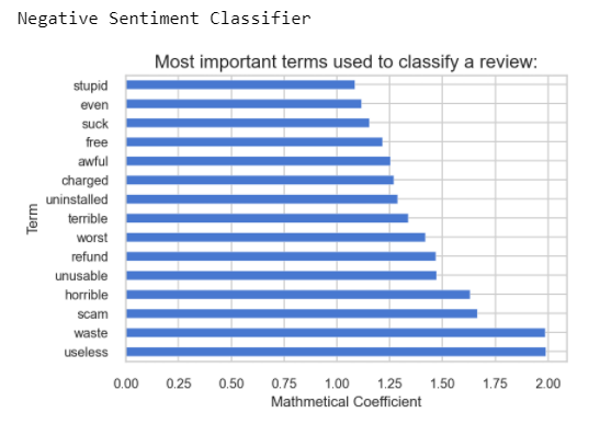

Well, that makes sense. You can see that the word 'useless' had the largest coefficient - meaning the word 'useless' is the most important word in classifying a review as bad... just ahead of 'waste'. This was insightful. But it also didn't tell me much as to what was so bad... or useless... which is what led me further down the road of removing these kinds of words and then doing some cluster analysis.... LDA ... and that's where I remember the outcomes more. To get there though, I had to classify the text first. Then, to remove all the non-additive words I had to know what they were. The coefficients from scikit learn's Linear Support Vector Classification model was the ticket, and plotting them helped me extract meaning as well as build a list. I'm glad I looped back to remember how I got there. After taking another look, I might improve my model to see if I could get a better outcome.