Evaluating a Recurrent Neural Network:

When you hear the term neural network - it's intimidating. It seems complicated. It is - but if you relate it back to a system that works like a brain it might simplify things.

In deep learning models called neural networks used in data science, synapses (think like in a brain) connect neurons in layers - multilayer perceptrons. These connections or synapses are informed through what’s called backpropagation and strengthen or weaken as they pick up on patterns in the data. How well this validation compares with how the model responds to the data it's learning on help inform how well a model is working and is a first step in how your model works.

Ok that was a lot. Have I already lost you?? Let me back it up and break it down a little. The idea of this post is to not make anyone an expert, but rather help give a high-level overview of how to begin to evaluate a neural network. First, a high-level overview of what it is and how it works.

A neural network is made up of a bunch of connected neurons.

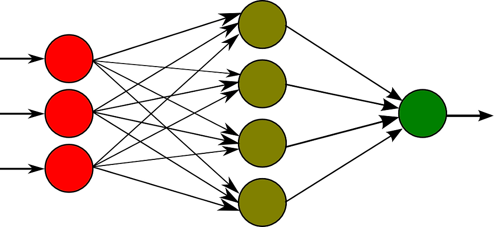
A neuron is the building block of a neural network. It takes in numeric data (it cant be categorical data for example categorizing something like 'male' or 'female'. It has to be numeric- a 0 or a 1. Like a biological neuron, if the data conditions meet a minimum threshold, it uses an activation function and gives the output. Each input and output is given a 'weight' or how strongly to rely on this connecting feature. In the example below the weight could be interpreted as how thick the lines are.

A multilayer perceptron is a bunch of layers made up of these neurons connected together. In the image below the input is the red layer, the 'hidden layer' is the lighter green in the middle, and the last single green dot is the out put layer.

image cred

Through 'training' the network - or passing data with a known outcome and comparing them to expected outcomes, an error is calculated. These errors are passed back through the network one layer at a time through that backpropagation process I mentioned in the beginning. Each time this process happens it's called an epoch. The lower the error is, the better the model is. This is one way to evaluate how the model is working.

This is a ton of information to keep track of, and it can compound rapidly. Each epoch adjustments are made to minimize the loss rate. If it happens too quickly and how much the model adjusts - called the 'step size' is too big, an optimal setting might be skipped over. If it happens too slowly, we might not realize an optimal setting because it would take too long to go through enough epochs. This can be controlled with what's called a learning rate. The learning rate adjusts what increment to increase or decrease the suggested changes. It helps with 'overtraining' and 'undertraining' a model. If a model learns the data really well it would perform better on the validation. This demonstrates that it's overtrained - it knows how to solve the problem too well. It's like memorizing the answers so you can answer them even before you're asked. If it's undertrained it means it could simply perform better. This is the basics of evaluating how well your model works.

Perhaps we could go through an example I used in combination with natural language processing to classify toxic language. The process of turning text into numeric values is called tokenization and is necessary in modeling text in the process of natural language processing or NLP. If you remember from a little further up this page, we need numeric values for this model. Keras is an open-source tool for building neural networks and has a library I found to be especially helpful for deep learning and found out that they have a package for tokenizing.

Before this, many preprocessing steps used in natural language processing NLP. I detail preprocessing in this blog, but will skip these details - I'm trying to keep things high level in this post. You can also do a lot of this within Keras' Tokenizer - live and learn 'sigh'.

from keras.preprocessing.text import Tokenizer
max_features = 2000
tokenizer = Tokenizer(num_words=max_features)
tokenizer.fit_on_texts(list(X_train))
#try texts_to_matrix
list_tokenized_train = tokenizer.texts_to_sequences(X_train)
list_tokenized_test = tokenizer.texts_to_sequences(X_test)

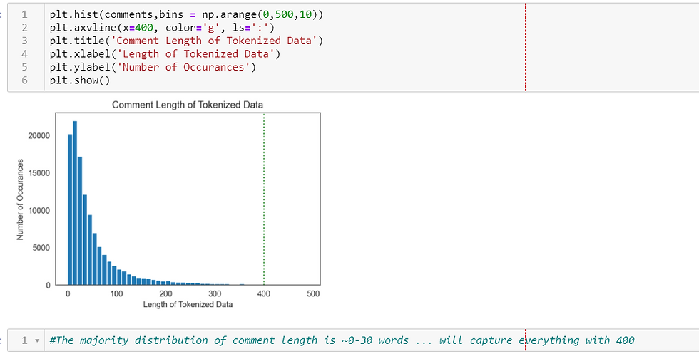
Once the data was tokenized, I looked to see how long these comments were. This is important since we tell our model how long each 'vector' is when we feed it into our model.

We can visualize this with a histogram. This shows us very clearly that the most common length of a comment was between 0-30 tokens. It also suggests that a length of 400 would capture most of the data.

I 'padded' the sequences, again using the Keras API, and looked at the shape - perfect.

from keras.preprocessing.sequence import pad_sequences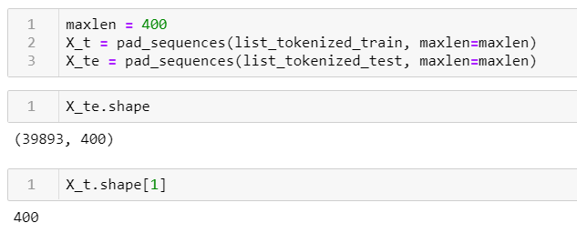

With Keras, you need to instantiate your model - or create a working copy of it:

van_model = Sequential()

Then build our multi-layer perceptron model. I won't go into the details, or how to tune all the hyperparameters of this model in this post since we're trying to focus more on a high-level evaluation. Hyperparameters would include how many epochs, or learning rates that I mention above among other things. If you can't wait, you can look at the documentation:

van_model.add(Dense(10, activation='relu', input_shape=(X_t.shape[1],) ))
van_model.add(Dense(6, activation='sigmoid'))

Then you compile it:

van_model.compile(optimizer='sgd',
              loss='binary_crossentropy',
              metrics=['accuracy'])

Finally, you fit the model. Here's where I tell it to go for 10 cycles feeding the training data through, backpropagation and updating the model appropriately or if you remember from when I explained it above, epochs:

van_history = van_model.fit(X_t, y_train, epochs=10,
                            batch_size=200,
                            validation_split=.2)

To see what we came up with in terms of accuracy and loss, I wrote the function below to plot the learning curves for the models. I'm extremely visual, so plotting the outcomes help a person like me a lot. What I was looking for was how the model's training data did in comparison with the validation data over the course of each epoch. Specifically - how accurately it performed and the loss. These two things help to identify if my model is under or overfit and what the loss looks like. The basics for evaluating a neural network.

def plot_loss_acc(history):
    import matplotlib.pyplot as plt
    %matplotlib inline 

    acc = history.history['accuracy']
    val_acc = history.history['val_accuracy']
    loss = history.history['loss']
    val_loss = history.history['val_loss']
    epochs = range(1, len(acc) +1)
    plt.plot(epochs, acc, label='Training accuracy')
    plt.plot(epochs, val_acc,color='g', label='Validation accuracy')
    plt.title('Training and validation accuracy')
    plt.legend()
    plt.figure()
    plt.plot(epochs, loss, label='Training loss')
    plt.plot(epochs, val_loss, color='g' , label='Validation loss')
    plt.title('Training and validation loss')
    plt.legend()
    plt.show()

In these plots, we can compare to see how well the training and validation accuracy and loss compare to each other to inform if something is over or undertrained. In a perfect world, we'd have high accuracy, low loss AND the validation and training would 'match' one another.

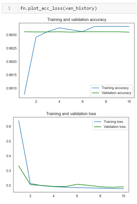
On the first very small and simple model, we can visually see that this model wasn't great. Even though the accuracy is high by the 10th epoch, the validation accuracy barely changes at all over time - it's a straight green line. This might mean that the learning rate might be too quick it's overtrained. For loss, it matches up right around 4 epochs. Over the next several rounds we'd need to make some adjustments.

To probably give too much background, this was a pretty hairy dataset with 6 overlapping classifications of toxic language. Six ways people classified toxic langue - like toxic, insulting, threatening as examples. It also had hyper imbalanced targets. Hyper imbalance just means that there was a lot of data to train the model in some of the 6 categories but barely data to train the model in others. But, after several attempts and implementing a few tricks to address this hyper imbalance, I got a model that turned out to be fairly decent. I knew this by visualizing the accuracy and loss of the training and validation using the function I wrote.

Here's the model I used. Don't get lost in the code. Stay with me on a high level. I shared it with you because it just gives an idea that I went from two lines of a fairly simple model to more advanced with a lot of 'tweaking'.

rnn_last = Sequential()
embedding_size = 128

rnn_last.add(Embedding(max_features, embedding_size))
#adding LSTM layer to help 'forget' then pooling
rnn_last.add(LSTM(50, return_sequences=True,name='lstm_layer'))        
rnn_last.add(GlobalMaxPool1D())
rnn_last.add(Dropout(0.2))  
rnn_last.add(Dense(25, kernel_regularizer=regularizers.l2(.0001),activation='relu'))
rnn_last.add(Dense(6, activation='sigmoid'))

rnn_last.compile(loss=BinaryFocalLoss(gamma=2),
                  optimizer='adam',
                  metrics=['accuracy'])

## WARNING ⏰ 70 Min+ RunTime ⏰
#fit the model
timer = fn.Timer()
timer.start()
history_lst = rnn_last.fit(X_t, y_train, epochs=20,  batch_size=300, 
                        callbacks=early_stopping, validation_split=0.3)
timer = timer.stop()

...and plotted the results:

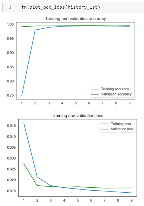
Here you can see despite being slightly undertrained, the model converges in terms of accuracy and loss right around 4 epochs. This model most accurately was able to identify the toxic language overall - 98% accurate is pretty good. I looked more closely at other metrics that could better flag each of the individual classes of toxic language.

While the overall accuracy of this model is pretty great - it's because it was across all categories. Remember how I mentioned some of the categories had very little data in them? Now that I see that the model is performing pretty well at a high level, I needed to see how they performed individually.

Armed with the basic insight into how the model was performing, I looked a little deeper with the use of a confusion matrix. Confusion matrices illustrate what we've become too familiar with since covid19 reared its head - true positive and true negative rates. True positives are those that the model predicted to be in the target class. True negatives are those that the model predicted to not be in the target class. What we're looking for is the ability to identify True Positives for each - or look at recall - this would be a better metric in this case.

In this case, there is some good news and some bad news in this model used to identify toxic language. The good news: some of the classes had so few examples to train my model - meaning the category of 'identity hate' and 'threats' happened very infrequently... making it difficult for my model to learn characteristics of these comments. This brings me to my bad news: values of 0 for recall to identify these categories. To do change this, we'd need to get more data to train my model on. This is another chapter and I am beginning to ramble on outside of the scope of what I'd set out to do today.

The main idea here was to take a look from a high level to evaluate how good the model was performing based on accuracy and loss. Once we get results with high accuracy and low loss, we can begin to dive deeper into more useful, detailed metrics like true positive and true negative rates. I hope this very high-level overview gave you an idea of how to begin to evaluate a neural network.

If you're interested in the project go take a look. I'll warn you - there's some pretty toxic language out there. Please please keep in mind I didn't create the dataset, did not create or support any of the sentiment captured in the toxic language. However, I feel it important to observe it in order to evaluate findings. It was super interesting and ultimately comforting to know that while unfortunately, toxic language exists, there was a very limited amount of it overall - even though it negatively impacted my model - :-).

Let me know what you think. If someone showed you these learning curve plots, could you tell the difference between a high or low-performing model? Have you used a neural network before? What did you build it to predict? What were your challenges?