Tuning SARIMA Time Series:

In my prior post on time series, I covered at a high level the various components of a time series - noise, seasonality, and trends. I covered stationarity in data and it's importance in the ability to predict future values that are dependent on time.

On a high level the process for building a time series model looks like this:

1. Detrend the time series (my fave is by using differencing). ARMA models represent stationary processes, so we have to make sure there are no trends in our time series. The package we'll use today uses differencing automatically.

2. Look at autocorrelation and in some cases partial autocorrelation of the time series

3. Decide on the AR, MA, and order of these models

4. Tune / Fit the model to find the best parameters for prediction.

5. Evaluate the model - and perhaps revisit step 4.

Let's dive in!

Step 1:

First, we load the dataset and set the index with the time value. We'd normally detrend the data, but the package we're using today uses differencing so we can skip the Dickey-Fuller test for now. Let's just load it and get it into a time-series format:

#load the dataset
df = pd.read_csv("https://raw.githubusercontent.com/jbrownlee/Datasets/master/monthly_champagne_sales.csv")

#changing Month to datetime
datetime = pd.to_datetime(df['Month'])

#setting the datatype to datetime
df.index = datetime

#dropping the column that's no longer necessary
df.drop(columns="Month", inplace=True)

#creating a timeseries using sales and dates
ts = pd.Series(df['Sales'].values, index=datetime)

At this point, my dataset has been prepared for use and is ready to begin exploring a little bit.

Step 2:

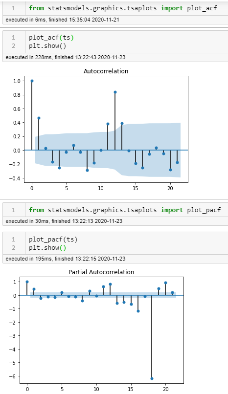
Autocorrelation and Partial Autocorrelation uses lags to reveal seasonality of data. Statsmodels.graphics.tsaplots library has a great package for this:

The ACF shows the autocorrelation between one observation and the one at the prior time step that includes direct and indirect dependence information.

On both plots, we're looking for the points that occur before the confidence interval indicated by the dark blue shading. Where the peaks trail off should give us an idea of the order. In both cases here, I count 1 as the first and 12 being highly correlated (not shocking) in both cases, but on the partial, I see 8, 18 as well. Interesting.

Let's look at some other indicators of seasonality as well.

Another tool I mentioned in my prior post that Pandas API uses is handy as well.

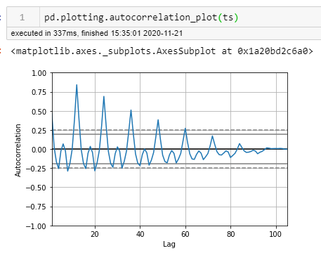
Here I count six points prior to where it falls below the confidence interval at intervals of 12 months.

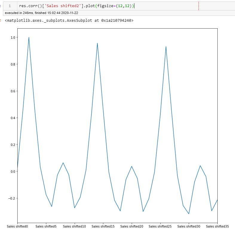
I'd also just used the .shift() function to see general correlations. Patterns of 2, 6, and 12 are apparent in all of these. A LOT to take into consideration and to try every single one out to pick the best parameter could take a ton of time.

If you haven't guessed...

I like EDA - Exploratory Data Analysis. One more visual to confirm and that really in my mind reveals patterns better than any so far:

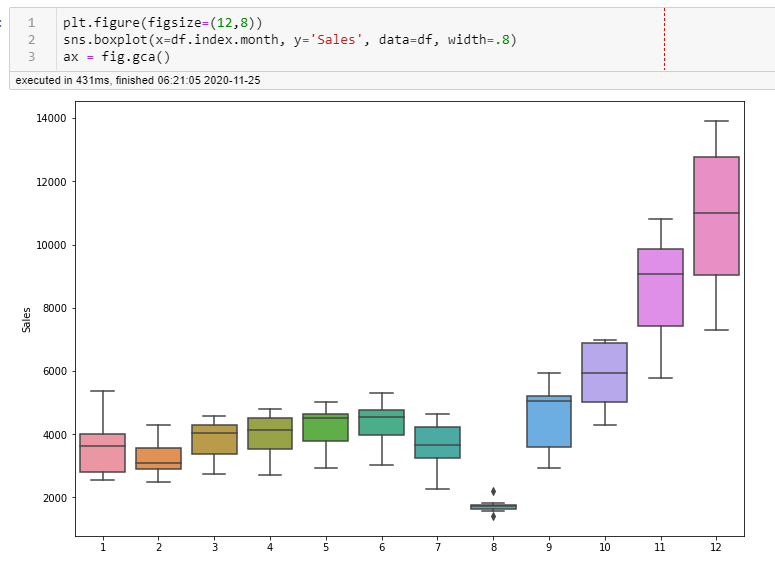
Patterns of 6, and 12 are apparent in all of these. Also, in this visual, you can see that in the 8th month of each year, sales are really low. A LOT to take into consideration and to try every single one out to pick the best parameter could take a ton of time.

Step 3:

Evaluation of the ARIMA / SARIMA models:

There are three basic parameters to tune in ARMA / ARIMA (S is for seasonal) models:

1. AR - Number of AR (Auto-Regressive) terms (p) will tell you the percent of a difference you need to take.

2. I = Number of Differences (d) today's difference versus yesterdays

3. MA -Number of MA (Moving Average) terms (q) is a past error multiplied by a coefficient.

These three distinct integer values, (p, d, q), are used to parametrize ARIMA models. Because of that, ARIMA models are denoted with the notation ARIMA(p, d, q). Together these three parameters account for seasonality, trend, and noise in datasets:

• (p, d, q) are the non-seasonal parameters described above.

Then we take into account seasonal parameters:

• (P, D, Q) follow the same definition but are applied to the seasonal component of the time series.

• (s) or the seasonality/periodicity or number of steps of the time series (4 for quarterly periods, 12 for yearly periods, etc.).

Together, the notation for a SARIMA model is specified as:

SARIMA(p,d,q)(P,D,Q)s

Statsmodels SARIMAX library does a lot of the heavy lifting and is what I'll be using. It implements each coefficient for each parameter. We may have some AR terms, some MA terms, it all depends on the specific series. This library uses differencing (my fave), and the X allows for exogenous features to be accounted for as well which I won't get into today, but if you're interested go here.

With SARIMAX the basic steps for creating a model:

# specify training data
data = ...
# define model
model = SARIMAX(data, order=..., seasonal_order=...)
# fit model
model_fit = model.fit()
# one step forecast
yhat = model_fit.forecast()

Finding the best parameters is important for accurate forecasting, a good starting place is by using the pacf and acf plots, as well as using a grid-search:

#creating my variables for (p,d,q)
p = d = q = range(0,2)
pdq = list(itertools.product(p,d,q))

#creating a list iterating through each combo and adding seasonality
pdqs = [(x[0], x[1], x[2], 12) for x in list(itertools.product(p,d,q))]

#creating a gridsearch to find lowest aic for model

ans = [['pdq', 'PDQ', 'aic']]

# SARIMA model pipeline
for arma in pdq:
    for sarma in pdqs:
        #there will probably be errors, so use of try and except:  
        try:
            mod = sm.tsa.statespace.SARIMAX(tstrain, order=arma,
                                            seasonal_order=sarma, 
                                            enforce_invertibility=False,
                                            enforce_stationarity=False)
            results = mod.fit()
            
            ans.append([arma, sarma, results.aic])
        except:
            continue

mod_aic_df = pd.DataFrame(ans[1:], columns=ans[0])

and then I sort the aic values to find the smallest values of aic:

Results here show that the best parameters for pdq:

0 - no autoregressive term

1- use one time lag

1- have one component for the moving average

Results here show that the best parameters for pdq:

1 - no autoregressive term

1- use one time lag

1- have one component for the moving average

12 - use 12 months as our larger seasonality

Step 4 Building and Tuning:

Using these parameters, I build my model:

best_pdq = (0, 1, 1)
best_PDQS = (1, 1, 1, 12)

mod1 = sm.tsa.statespace.SARIMAX(tstrain, order=best_pdq,
                                seasonal_order=best_PDQS, 
                                enforce_invertibility=False,
                                 enforce_stationarity=False)
results1 = mod1.fit()

We have results. Now it's time to evaluate the model. Since this is essentially a regression we are looking for the same values like mean square error, p values etc.

Linear regressions require the data to be normal. A quick and dirty way is to just run a normal test on this:

from scipy.stats import normaltest
resid1 = results1.resid
print(normaltest(resid1))

NormaltestResult(statistic=77.16580708641763, pvalue=1.7524994703303525e-17)

Nice p-value! Super tiny. This means that there's that percent chance that this result is due to error that the data is normal. We're on the right track!

Step 5:

When I predict the future values, things don't look good for this company. You can see that my model picked up on the downward trend.

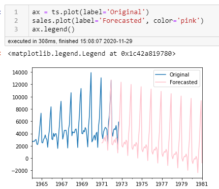
I think I might need some more tuning. Let's look at the root mean squared error:

expected = ts['1971':'1972']
predicted = sales['1971':'1972-09-01']
from sklearn.metrics import mean_absolute_error, mean_squared_error

mean_absolute_error(expected, predicted)
1262.5097591470185

np.sqrt(mean_squared_error(expected, predicted))
1409.0154296190246

Yep. These values are fairly high. I will when I have time I'll go back to step 3 and gridsearch some other values in my ranges including values of 2, 6 and 12. We'll see if things can improve. Let's hope for the sake of this champagne company it does!

Additional reading: https://www.researchgate.net/post/How-does-one-determine-the-values-for-ARp-and-MAq